|
Geometric model of muscle contraction |
|
Izidor Hafner, Boštjan Šimunič, Vojko Valenčič, Srdjan Djordjević, Peter Stušek*, Gregor Žnidarič* Faculty of electrical engineering Tržaška 25, 1000 Ljubljana *Biotehnical Faculty Slovenija email: izidor.hafner@ fe.uni-lj.si |
Abstract--We use a function transformation that leaves volume unchanged as the basis for geometric model of muscle contraction. The model is built after making an experiment on a frog leg muscle under single electrical stimulus.
Index Terms—Geometric model, muscle,
electric stimulus.
I.
INTRODUCTION
Geometric models of different skeletal muscle with mechanochemical properties
have been used for some time [1]. Pure geometric model can be used to calculate
contraction from radial displacement or vice versa. At Faculty of electrical engineering a new
non-invasive method called tensiomiograpy (TMG) has been developed [3]. The
method enables selective measurements of particular muscles. This method is based
on magnetic displacement senzor detecting the muscle belly enlargement in
radial direction. The figure 1 shows
the basic principle of TMG.
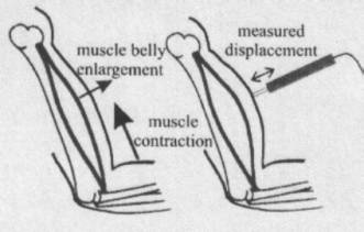
Fig. 1.
Principle of TMG method
In studying a muscle as geometric object we limit to simple geometric shapes. This means that the radial cross section is an ellipse. We make also a natural presupposition that the volume of a muscle remains unchanged during contraction.
II. EXPERIMENT
On frog’s (Bufo bufo) leg muscle (gastroncnemius) strained with almost constant force of 0.34 to 0.42 N (isotonic conditions) a single electric stimulus was enforced. The muscle contracted from 25 mm to 18 (or 17) mm. The radial enlargement from top view was from 6 to 8 mm (figures 2, 3). The radial enlargement from side view was from 5.75 to 6.5 mm (figures 4, 5). The difference of radial enlargements among both views was significant. The volume of the muscle was 400 mm3. The experiment has been carried out at Biotehnical Faculty.
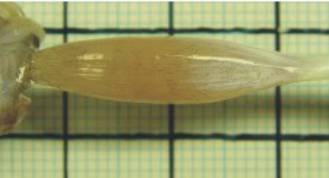
Fig. 2. The
relaxed muscle, top view
Fig. 3. The
contracted muscle, top view
Fig. 4. The
relaxed muscle, side view
Fig. 5. The contracted muscle, side view
III. GEOMETRIC MODEL
It is reasonable to suppose that a cross section is an ellipse. For 2D model (figures 6, 7) we take a circle as cross section where the radius is geometric mean of ellipse’s half-axes. So the model is then a solid determined by surface of revolution. For a curve that forms the surface we take part of max(1- x2/c2)f. Max is maximum value of the function on interval [-c,c], Zeros –c and c are estimated by drawing tangents at end points of the muscle. Parameter f (in our case it equals 1.5) is determined by calculating the volume of the solid from formula
![]()

Fig. 6. A
model of muscle (contraction)
Fig. 7. A model of muscle (relaxation)
The figure 8 shows both (enlarged) cross sections.
Fig. 8. The
model’s average cross sections
Parameters a in b are the beginning and the end of the muscle.
We know that f(mx), m>1, means shrinking of function f along x axis for factor m. Note that function g(x)=Ömf(mx) determines the same volume on interval [a/m,b/m] as f(x) on [a,b].
Proof: t=mx,
dt=mdx
![]()
In our case the shrinking factor m=25/18=1.39 (or 25/17=1.47). This means that the average radial enlargement equals Öm=1.18 times average radius of the beginning state of the muscle.
Suppose the cross section is an ellipse with half-axes y and z.
Then the volume equals

If the radial enlargements in directions of y and z axes are h and k respectively, then hk=m. In our case h=1.33, k=1.13. The product is 1.5. The relative error 0.11/1.5=0.07 (or 0.03/1.5=0.02) occurs because the real muscle is not as symmetric as we supposed (figure 9).
Fig. 9. The
model’s cross sections
Using a function of type a(1-x2/c2)f has the advantage that the integral of its square can be calculated analytically. Also the maximum value a is achieved at x=0. Since there are only 3 parameters we can model only 3 quantities. We take volume, maximum end length of the muscle.
We experimented also with some other three parametric functions: ax(x-b)(x-c), a(1-x2/c2)/(1+bx2). The main problem of functions is to find critical points. Even in case of polynomials of degree more than 2 we get nonlinear equations and if the degree is more than 5, the first derivative has degree more than 4 and the equation f’(x)=0 is not solvable (by formula).
In some applications we can suppose that a muscle ends in a point (figure 1). An example of such application may be a web animation of muscle contraction. In such cases three parametric functions are quite adequate. Here are some shapes we get for different values of parameters a, c and f of the function
a(1-x2/c2)f.
Fig. 10. a=0.34, c=1.25, f=7
Fig. 11. a=0.34,
c=1.25, f=1
IV. Conclusion
Generally shapes of human or animal muscles are too complicated to be treated by mathematical formulas. In some cases a muscle has relatively simple form and it is possible to find a mathematical function that aproximate the muscle’s shape. We have investigated one such muscle, but generally the problem remains open.
References
[1] K. Akazawa, M. Yamamoto, K. Fujii, and H. Mishima, “A mechanochemical model for the steady and transient contractions of the skeletal muscle”, Jap. J. Physiol., 26,9-28,
[2] A. Belič, N. Knez, R. Karba, V. Valenčič, “Validation of the human muscle model”, Proceed. 2000 Summer Computer Simulation Conference, 16.-20. July 2000, Vancouver, British Columbia. Session 1: Issues on Whole Body Modeling.
[3] N. Knez, V. Valenčič, “Influence of impulse duration on skeletal muscle belly response”, Proceedings of the ninith Electrotechnical and Computer Conference ERK 2000, 21.-23. September 2000, Portorož, Slovenia, Ljubljana: IEEE Region 8, Slovenian section IEEE, 2000, Vol. B, pp. 301-304.